
The method, since 1990
Discrete rate simulation
A way to simulate lines that move product as a flow: bottles, cans, powder, liquid, grain. It models rates instead of individual items, so a model of a high-speed line runs in a fraction of the time and still captures every stop, starve and block. We created it, and we still use it.
What is discrete rate simulation?
Discrete rate simulation (DRS) is a form of discrete event simulation in which the thing that flows through the model is a rate, not a stream of individual items. A filler runs at a rate. A conveyor carries a rate. A tank fills at the difference between the rate coming in and the rate going out.
The model only does work when a rate changes. A machine breaks down, a buffer fills, a tank runs dry, a changeover starts, a shift ends. At each of those moments the model works out the new rate for every connected piece of equipment and then calculates when the next change will happen. Between events, nothing needs to be computed, because the flows are known.
Andy Siprelle created the method in 1990 under the name bulk flow simulation. It was later renamed discrete rate simulation, and discrete rate libraries or extensions are now part of all the major commercial simulation packages, including ExtendSim, AnyLogic and Siemens Plant Simulation.
Why rates instead of items?
Take a packaging line that fills product at high speed. A conventional discrete event model treats each container as its own item. Every container is created, moved, queued, filled, capped, labeled and packed, and each of those steps is an event the computer must schedule and process. The event count grows with every container the line makes.
Most of those events tell you nothing new. While the line is running smoothly, container 40,001 behaves exactly like container 40,000. What matters is when that smooth running stops, and how far the effect spreads up and down the line.
A rate model skips the repetition. For a high-speed system it can cut the events in a stretch of simulation from 40,000 steps to 2. That speed changes how the model gets used. You can run many replications, test many scenarios and check the model against history, in the time a conventional model takes to run a handful of cases.
Discrete rate vs. discrete event vs. continuous
The three approaches sit on a scale from fine detail to broad flow. The Fraunhofer Institute describes discrete rate as mesoscopic simulation, between microscopic item-by-item discrete event models and continuous models of flows.
| Discrete event | Discrete rate | Continuous | |
|---|---|---|---|
| What flows | Individual items, each with its own attributes | Rates of flow between pieces of equipment and storage | Quantities that change smoothly over time |
| When the model calculates | Every time an item moves or changes state | Only when a rate changes: a stop, start, full or empty | At every small time step |
| Best fit | Assembly, job shops, routing, items with individual identity | High-speed packaging, food and bulk lines, tanks, conveyors, make-store-pack plants | Chemical reactions, heat transfer, process control |
| Run speed on a high-volume line | Slow, because event counts grow with volume | Fast, because events grow with changes, not volume | Depends on the time step |
| Watch out for | Run times that make experiments impractical | Questions that depend on one specific item | Discrete stops and changeovers are awkward to represent |
None of these is better in general. A model of vehicle routing or an assembly plant where every unit carries its own options belongs in discrete event. A model of a line moving hundreds of containers a minute through accumulation conveyors belongs in discrete rate. Many real plants need both, and a good discrete rate tool will let you mix them: rate flow on the high-speed packing line, individual items for the pallets that come off the end.
Where discrete rate wins
High-speed consumer packaged goods lines
Filling, capping, labeling, case packing and palletizing lines run fast and stop often. Short stops matter because they add up, and because accumulation between machines decides whether a stop stays local or takes the whole line down. A rate model captures each stop and each buffer precisely without paying for every container.
Bulk flow
Powder, grain, liquid and other bulk material has no natural "item" at all. Forcing it into items means inventing a lot size and living with the error. A rate model handles it as it really is. Our first published model, in 1995, was a bulk manufacturing system.
Tanks, bins and silos
In-process storage fills and drains at the difference between two rates. A rate model knows exactly when a bin will fill or empty, so it can show when an upstream process will block, when a packer will starve, and what the storage is worth.
Conveyors and accumulation
Conveyors both move product and store it. Discrete rate models treat accumulation as the buffer it is, which is usually the question: how much conveyor, and where?
Make-store-pack plants and moving bottlenecks
When a making process feeds storage that feeds packing lines of different speeds, the bottleneck can move with the product mix. We call this the "slurp rate" problem: depending on the package size, the packing lines draw down in-process storage too fast or too slowly. Rate models are well suited to testing scheduling rules against it. In one coffee plant, a quality change inserted a new step between roasting and grinding, and the planning system could no longer build schedules that held up. A discrete rate model let the team conceive, test and verify a new scheduling algorithm that held up across demand scenarios.
Supply chains
The same idea scales up. Product moving between plants, warehouses and customers can be modeled as flows, which is why months of supply chain operation can run in minutes.
Worked example
How much buffer does a filling line need?
A question every packaging engineer faces, answered with a discrete rate model.
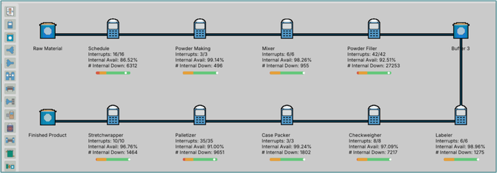
This model is a powder filling and packing line. Product is made and mixed, then flows through a powder filler, labeler, checkweigher, case packer, palletizer and stretchwrapper. Each machine carries its real stop history: the model shows every interrupt type, its internal availability and how many times it went down.
"Buffer 3" sits between the powder filler and the labeler. With no buffer, the two machines are tightly coupled. When one stops, the other stops at once. With a little buffer, the other stops a little later, or not at all if the first one restarts in time.
The question: how big should Buffer 3 be? More buffer usually means more throughput, which surprises people. But bigger bins and longer conveyors cost money and floor space, and at some point the returns shrink.
Reading the result
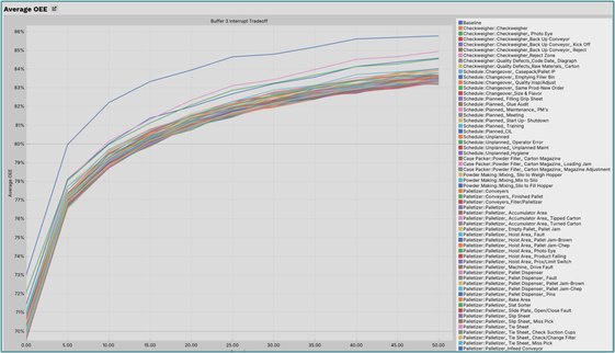
We ran a "buffer tradeoff" experiment that varies the capacity of Buffer 3. At zero, the buffer is just a pass-through and the filler and labeler are closely coupled. Each colored line is a scenario. The baseline, with every as-is failure switched on, hugs the bottom. Each of the other lines switches off one failure type to show what fixing it would be worth.
Every line follows the same shape. OEE climbs steeply with the first bit of buffer, then flattens. That knee is the answer to "how much?" And the gap between lines answers the other question: is it worth more to fix a particular failure or to buy more buffer?
A discrete rate model makes this experiment practical. Dozens of scenarios, each with many buffer sizes and replications, run quickly because the model only calculates when a rate changes.
History
Where discrete rate simulation came from
Andy Siprelle created bulk flow simulation in 1990 to model high-speed and bulk lines the way they actually run. SDI built it into libraries for Extend, the simulation package now called ExtendSim. Our original Bulk Flow (Rate) and Database libraries sold 700 licenses, and they became the base of ExtendSim's current Discrete Rate and Database libraries.
The first paper, "Modeling a Bulk Manufacturing System Using Extend," was presented by A. J. Siprelle and D. J. Parsons at the 1995 Winter Simulation Conference. "Simulation of Bulk Flow and High Speed Operations" by Siprelle and Phelps followed at WSC 1997, and the SDI Industry library was described at WSC 1998.
A second generation followed from others. Damiron and Nastasi described discrete rate simulation using linear programming in 2008, and Krahl described ExtendSim's discrete rate technology in 2009. Researchers at the Fraunhofer Institute later framed the approach as mesoscopic simulation, and in 2020 Fischel and Lange presented high-accuracy discrete rate and reliability modeling for plant OEE and throughput.
"SDI Industry's Discrete Rate Flow represents a breakthrough for modeling high-volume operations. Anything that can be expressed in terms of rates can be modelled more effectively than discrete event by using Discrete Rate Flow."
Darrell Starks, Simulation Consultant, Integral Solutions
Key papers
- 1995Modeling a Bulk Manufacturing System Using Extend
The first paper on bulk flow simulation.
- 1997Simulation of Bulk Flow and High Speed Operations
Bulk flow modeling applied to high-speed operations.
- 1998SDI Industry: An Extend-Based Tool for Continuous and High-Speed Manufacturing
The library that carried the method into client projects.
- 2008Discrete Rate Simulation Using Linear Programming
Related research: solving rate networks with linear programming.
- 2009ExtendSim Advanced Technology: Discrete Rate Simulation
Related research: the discrete rate engine in today's ExtendSim.
- 2020High Accuracy Discrete Rate and Reliability Modeling to Drive Improvement of Plant OEE and Throughput
Related research: a rate and reliability model checked against one plant's measured OEE.
Case studies
Discrete rate models at work
A chemical bagging operation, an olive plant and a packaging network, each modeled as flows.
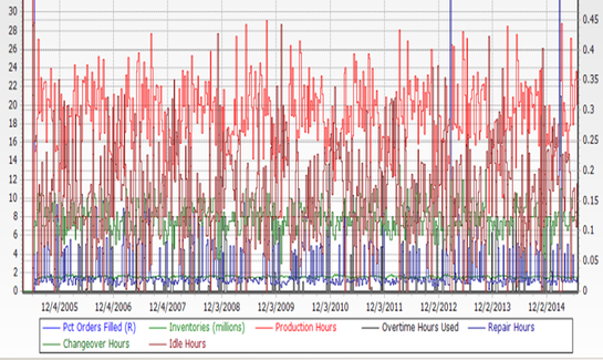
Chemical bagging lines: capacity vs. overtime
Weighing new bagging lines against overtime, and finding low-capital room to grow.
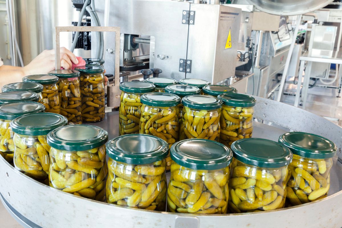
Olive plant capacity: 15% more throughput
Finding the real bottlenecks in an olive plant, and 15% more throughput from scheduling.
15% throughput improvement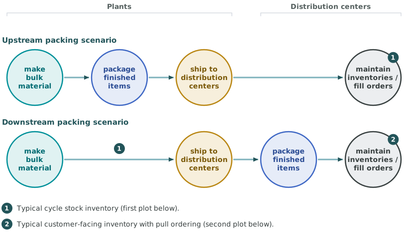
Packing at the DC: inventory vs. bulk stock
Should packaging move to the distribution centers? The answer, product by product.
Is discrete rate right for your line?
If your line runs fast, stops often and has accumulation between machines, probably yes. If each unit carries its own route or options, a discrete event model may fit better, and we build those too.
Tell us what the line makes, how fast it runs and what decision you are facing. We will tell you which approach fits and what a model could show you.
Common questions a rate model answers
- How much accumulation between two machines, and where?
- Which stops are worth fixing first?
- What will a faster filler actually add to output?
- Can the packing lines keep up with the new product mix?
- How big do the tanks, bins or silos need to be?
Tell us your problem
What would happen if you changed it?
Describe the decision in front of you. We'll tell you whether a model can answer it, and what it would take.
- A straight answer on whether simulation is the right tool
- Which tool fits, even if it isn't one we use every day
- A rough scope and timeline, before any commitment